Pull into Place (PIP) Step-by-Step Tutorial

The most up-to-date version of this tutorial is available on GitHub.

Model system

For the purposes of this tutorial, we will be examining Ketosteroid isomerase (KSI), which is a model enzyme that catalyzes the rearrangement of a double bond in steroid molecules. Asp38 is the key catalytic residue responsible for taking a proton from one site and moving it to another:

The enzyme is 200x less active when Asp38 is mutated to Glu (D38E), even though Asp and Glu have the same carboxyl (COOH) functional group. The difference is that Glu has one more carbon in its side chain, so the COOH is shifted out of position by just over 1Å. This demo will show everything you would need to do to use Pull Into Place (PIP) to redesign the active site loop to correct the position of the COOH in the D38E mutant.

Before you start

This demo will demonstrate how to run each of the individual PIP stages. Output will be generated via extremely short trajectories to allow the commands to be run locally on a laptop. For a real problem, PIP will most likely need to be run on a large cluster (as described in the general PIP documentation).

You also need to have Rosetta compiled on your workstation. In general, PIP doesn’t care where Rosetta is installed; it just needs a path to the installation. This tutorial will assume that Rosetta is installed in ~/rosetta such that:

$ ls ~/rosetta/source/bin
...
rosetta_scripts
...

If your Rosetta installation location varies, you will need to change the ROSETTA= variable at the top of each run script to the correct location (the path should already be correct if you are using the tutorial virtual machine).

Finally, you need to download and extract the loop hash database we’ll be using (this is already done in the tutorial virtual machine). Save it (or symlink it) directly into this folder with the folder name loophash_db.

Input information

All of the required input files have already been generated for you, but here are descriptions of the relevant file types for your future reference:

Input PDB file: A structure containing the functional groups to be positioned.
This file should already be parse-able by Rosetta, which often means it must be
stripped of waters and extraneous ligands.

Loops file: A file specifying which backbone regions will be allowed to move.
These backbone regions do not have to be contiguous, but each region must span
at least 4 residues.

Resfile: A file specifying which positions to design and which positions to
repack. It is recommended to design as few residues as possible outside the loops.

Path to resfile: ~/ksi_inputs/resfile

Restraints file: A file describing the geometry you're trying to design.  In
Rosetta parlance, this is more often (inaccurately) called a constraint file.
Note that restraints are not used during the validation step.

Score function: A file that specifies weights for all the terms in the score
function, or the name of a standard Rosetta score function.  The default is
talaris2014.  That should be OK unless you have some particular interaction
(e.g. ligand, DNA, etc.) that you want to score in a particular way.

Build script: An XML Rosetta script that generates backbones capable of
supporting the desired geometry.  The default version of this script uses KIC
with fragments in "ensemble-generation mode" (i.e. no initial build step).

Design script: An XML Rosetta script that performs design (usually on a fixed
backbone) to stabilize the desired geometry.  The default version of this
script uses fixbb.

Validate script: An XML Rosetta script that samples the designed loop to
determine whether the desired geometry is really the global score minimum.  The
default version of this script uses KIC with fragments in "ensemble-generation
mode" (i.e. no initial build step).

Flags file: A file containing command line flags that should be passed to every
invocation of Rosetta for this design.  For example, if your design involves a
ligand, put flags related to the ligand parameter files in this file.

Build initial backbone models

The first actual design step in the pipeline is to generate a large number of backbone models that support the desired side chain geometry. This will be done by running a flexible backbone simulation while applying the restraints we added to the workspace.

You can control which loop modeling algorithm is used for this step by manually editing build_models.xml. The current algorithm is loophash KIC (kinematic closure) , which samples conformations from a database of loop conformations hashed based on loop take off and ending points.

With the fast flag, which dramatically reduces both the number and length of the simulations, this step should take a few minutes. This (or similar) flags should not be used for production runs, but will continue to use it throughout this demo with the idea that your goal is just to run through the whole pipeline as quickly as possible.

Once the simulations finish, we can download the results to our workstation and visualize them

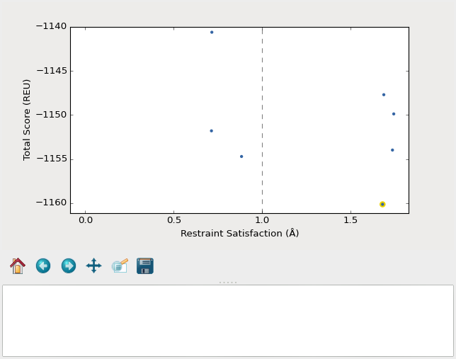
A screenshot of the plot_funnels GUI used in the full PIP pipeline.

Remember that the purpose of this step is to generate physically realistic models with the geometry we want to design. These two goals are somewhat at odds with each other, in the sense that models that are less physically realistic should be able to achieve more ideal geometries. We can use the displayed score vs. restraint satisfaction plot to judge how wells these two goals were balanced. If too many models superimpose with the restraints too well, the restraints might be too strong. If too few models get within 1Å of the restraints, they might be too weak. You can tune the weights of the restraints by manually editing restraints.

Task 1: Run the build_models.sh script

Stabilize good backbone models

The next step in the pipeline is to select a limited number of backbone models to carry forward and to generate a number of designed sequences for each of those models. It’s worth noting that the first step in the pipeline already did some design, so the purpose of this step is more to quickly generate a diversity of designs than to introduce mutations for the first time.

Task 2: Run the design_models.sh script

Validate good designs

You could have hundreds of thousands of designs after the design step, but it’s only really practical to validate about a hundred of those. Due to this vast difference in scale, picking which designs to validate is not a trivial task.

PIP approaches this problem by picking designs with a probability proportional to their Boltzmann-weighted scores. This is naive in the sense that it only considers score (although we are interested in considering more metrics), but more intelligent than simply picking the lowest scores, which tend to be very structurally homogeneous.

In a production run, PIP will open a window to show you how the scores are distributed and which were picked. As the command suggests, it worth looking at the cumulative distribution function (CDF) of the Boltzmann-weighted scores to make sure it’s neither too flat nor too sharp. This is a subjective judgment, but one good rule of thumb is that the designs being picked (represented by the circles) should be mostly, but not exclusively, low-scoring. The example CDF below looks about like what you’d want:

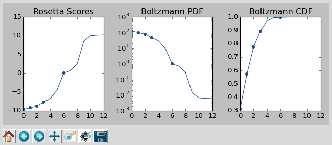
A screenshot of the 06_pick_designs_to_validate GUI.

A production validation step consists of 500 independent loop modeling simulations for each design, without restraints. We now will use the standard loop modeling algorithm KIC (instead of loophash KIC as in the initial build step).

Task 3: Run the validate_designs.sh script

Visualize designs

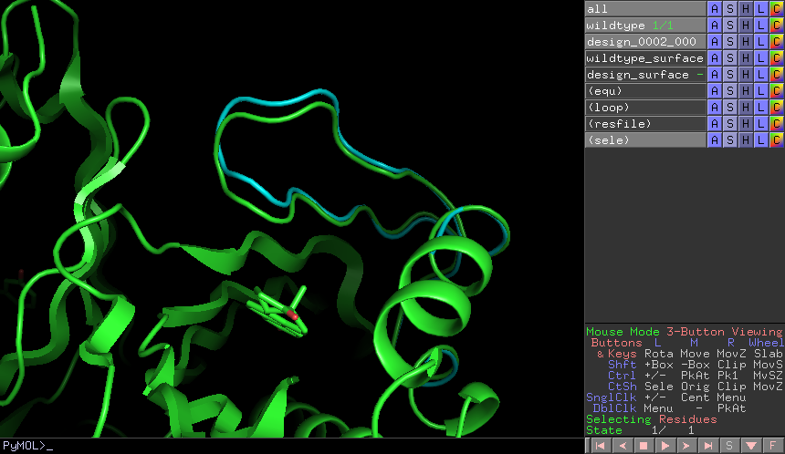
A screenshot of the PyMOL scene created by the compare_to_wildtype.sho script in the full pipeline.

We provide a plugin script that visually compares wild type with mutant structures. The plugin’s philosophy is to focus on each mutation one-at-a-time to try to understand what interactions the wild type residue was making and how those interactions are (or are not) being accommodated by the mutant residue. Visit this page for instructions on how to install and use wt_vs_mut.

Task 4: Use the wt_vs_mut PyMOL script to compare the output structure from the validation step validate_designs_KSI_D38E_0001.pdb with the wild type crystal structure KSI_WT.pdb. Follow the wt_vs_mut instructions to load the PyMOL visualization plugin (this is already installed in the tutorial virtual machine).

• In your terminal, launch PyMOL and load the two structures: pymol 4l7k_wt.pdb validate_designs_KSI_D38E_0001.pdb
• In PyMOL’s terminal:

run /path/to/wt_vs_mut.py (is /home/winter/TK/wt_vs_mut/wt_vs_mut.py in the virtual machine)
hide all
show car
show sticks, chain Y and not h.
align validate_designs_KSI_D38E_0001 and chain Y, KSI_WT and chain Y
wt_vs_mut KSI_WT, validate_designs_KSI_D38E_0001

Discussion questions

1. Did you find any mutations in your inspection of your validated design (from step Validate designs) that might actually make sense? (Note: we wouldn’t expect this to occur after such short simulations, but it is possible).
2. Did you find any mutations that definitely do not look good?

Compare design structures

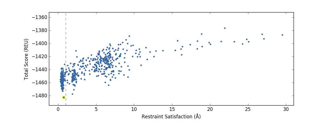
We will now compare the validated designs PDB you generated in a short simulation (validate_designs_KSI_D38E_0001.pdb) with designs generated from a full run of the PIP protocol.

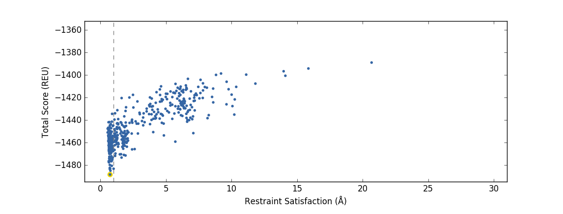
An example of a validation PIP run that produces a good design funnel, where the singular energy minima (as measured in Rosetta Energy Units) coincides with highest restraint satisfaction.

An example of a validation PIP run that produces a bad design funnel with multiple energy minima.

Task 5: Examine the structures sample_output/output_A.pdb.gz, sample_output/output_B.pdb.gz, and your validate_designs_KSI_D38E_0001.pdb output, using whatever structure visualization methods you prefer. Can you determine if output structure “A” or output structure “B” corresponds to the good validation funnel above?