Rescue the D38E mutation in KSI

Ketosteroid isomerase (KSI) is a model enzyme that catalyzes the rearrangement of a double bond in steroid molecules. Asp38 is the key catalytic residue responsible for taking a proton from one site and moving it to another:

The enzyme is 200x less active when Asp38 is mutated to Glu (D38E), even though Asp and Glu have the same carboxyl (COOH) functional group. The difference is that Glu has one more carbon in its sidechain, so the COOH is shifted out of position by just over 1Å. This demo will show everything you would need to do to use Pull Into Place (PIP) to redesign the active site loop to correct the position of the COOH in the D38E mutant.

Note

This demo assumes that you’re running the Rosetta simulations on the QB3 cluster at UCSF. If you’re using a different cluster, you may have to adapt some of the commands (most notably the ssh ones, but maybe others as well). That said, I believe the pull_into_place commands themselves should be the same.

Before you start

Before starting the demo, you will need to install PIP on both your workstation and your cluster. See the installation page for instructions. If you installed PIP correctly, this command should produce a lengthy help message:

$ pull_into_place --help

You also need to have Rosetta compiled on both your workstation and your cluster. See the Rosetta section of the installation page for instructions. In general, PIP doesn’t care where rosetta is installed; it just needs a path to the installation. This tutorial will assume that rosetta is installed in ~/rosetta such that:

$ ls ~/rosetta/source/bin
...
rosetta_scripts
...

Finally, you need to download the example input files we’ll be using onto your cluster. If your cluster has svn installed, you can use this command to download all these files at once:

# Run this command on ``iqint`` if you're using the QB3 cluster.
$ svn export https://github.com/Kortemme-Lab/pull_into_place/trunk/demos/ksi/inputs ~/ksi_inputs

Otherwise, you can download them by hand onto your workstation and use scp to copy them onto your cluster. You can put the input files wherever you want, but the tutorial will assume that they’re in ~/ksi_inputs such that:

$ ls ~/ksi_inputs
EQU.cen.params
EQU.fa.params
KSI_D38E.pdb
KSI_WT.pdb
compare_to_wildtype.sho
flags
loops
resfile
restraints

Set up your workspaces

Our first step is to create a workspace for PIP. A workspace is a directory that contains all the inputs and outputs for each simulation. We will call our workspace ~/rescue_ksi_d38e and by the end of this step it will contain all the input files that describe what we’re trying to design. It won’t (yet) contain any simulation results.

We will also use workspaces to sync files between our workstation and the cluster. The workspace on the cluster will be “normal” and will not know about the one on our workstation. In contrast, the workspace on our workstation will be “remote”. It will know about the one on the cluster and will be able to transfer data to and from it.

Note

Pay attention to the ssh chef.compbio.ucsf.edu and exit commands, because they indicate which commands are meant to be run on your workstation and which are meant to be run on the cluster.

The ssh shef.compbio.ucsf.edu command means that you should log onto the cluster and run all subsequent commands on the cluster. The exit command means that you should log off the cluster and run all subsequent commands on your workstation. If you get errors, especially ones that seem to involve version or dependency issues, double check to make sure that you’re logged onto the right machine.

First, create the “normal” workstation on the cluster:

$ ssh chef.compbio.ucsf.edu   # log onto the cluster
$ pull_into_place 01 rescue_ksi_d38e
Please provide the following pieces of information:

Rosetta checkout: Path to the main directory of a Rosetta source code checkout.
This is the directory called 'main' in a normal rosetta checkout.  Rosetta is
used both locally and on the cluster, but the path you specify here probably
won't apply to both machines.  You can manually correct the path by changing
the symlink called 'rosetta' in the workspace directory.

Path to rosetta: ~/rosetta

Input PDB file: A structure containing the functional groups to be positioned.
This file should already be parse-able by rosetta, which often means it must be
stripped of waters and extraneous ligands.

Path to the input PDB file: ~/ksi_inputs/KSI_D38E.pdb

Loops file: A file specifying which backbone regions will be allowed to move.
These backbone regions do not have to be contiguous, but each region must span
at least 4 residues.

Path to the loops file: ~/ksi_inputs/loops

Resfile: A file specifying which positions to design and which positions to
repack.  I recommend designing as few residues as possible outside the loops.

Path to resfile: ~/ksi_inputs/resfile

Restraints file: A file describing the geometry you're trying to design.  In
rosetta parlance, this is more often (inaccurately) called a constraint file.
Note that restraints are not used during the validation step.

Path to restraints file: ~/ksi_inputs/restraints

Score function: A file that specifies weights for all the terms in the score
function, or the name of a standard rosetta score function.  The default is
talaris2014.  That should be ok unless you have some particular interaction
(e.g. ligand, DNA, etc.) that you want to score in a particular way.

Path to weights file [optional]:

Build script: An XML rosetta script that generates backbones capable of
supporting the desired geometry.  The default version of this script uses KIC
with fragments in "ensemble-generation mode" (i.e. no initial build step).

Path to build script [optional]:

Design script: An XML rosetta script that performs design (usually on a fixed
backbone) to stabilize the desired geometry.  The default version of this
script uses fixbb.

Path to design script [optional]:

Validate script: An XML rosetta script that samples the designed loop to
determine whether the desired geometry is really the global score minimum.  The
default version of this script uses KIC with fragments in "ensemble-generation
mode" (i.e. no initial build step).

Path to validate script [optional]:

Flags file: A file containing command line flags that should be passed to every
invocation of rosetta for this design.  For example, if your design involves a
ligand, put flags related to the ligand parameter files in this file.

Path to flags file [optional]: ~/ksi_inputs/flags

Setup successful for design 'rescue_ksi_d38e'.

Note

You don’t need to type out the full names of PIP subcommands, you just need to type enough to be unambiguous. So pull_into_place 01 is the same as pull_into_place 01_setup_workspace.

You may have noticed that we were not prompted for all of the files we downloaded. EQU.cen.params and EQU.fa.params are ligand parameters for centroid and fullatom mode, respectively. PIP doesn’t specifically ask for ligand parameter files, but we still need them for our simulations because we referenced them in flags:

$ cat ~/rescue_ksi_d38e/flags
-extra_res_fa EQU.fa.params
-extra_res_cen EQU.cen.params

The paths in flags are relative to the workspace directory, because PIP sets the current working directory to the workspace directory for every simulation it runs. Therefore, in order for these paths to be correct, we have to manually copy the ligand parameters files into the workspace:

$ cp ~/ksi_inputs/EQU.*.params ~/rescue_ksi_d38e
$ exit   # log off the cluster and return to your workstation

KSI_WT.pdb is the structure of the wildtype KSI enzyme and compare_to_wildtype.sho is a script that configures and displays scenes in pymol that compare design models against KSI_WT.pdb. PIP itself doesn’t need these files, but we will use them later on to evaluate designs. For now just copy them into the workspace:

$ cp ~/ksi_inputs/KSI_WT.pdb ~/rescue_ksi_d38e
$ cp ~/ksi_inputs/compare_to_wildtype.sho ~/rescue_ksi_d38e

build_models.xml, design_models.xml, and validate_design.xml are RosettaScripts that run the various simulations that make up the PIP pipeline. We don’t need to do anything with these files (they’re for a different tutorial) because the 01_setup_workspace command already copied default versions of each into the workspace. We could provide different scripts if we wanted to change any of the algorithms PIP uses — for example, if we wanted to use a less aggressive backbone move like Backrub for a smaller remodeling problem, or if we wanted to use a design method like HBNet to prioritize getting a good H-bond network — but for this tutorial the defaults are fine.

Now that the workspace on the cluster is all set up, we can make the “remote” workspace on our workstation that will link to it:

$ cd ~
$ pull_into_place 01 -r rescue_ksi_d38e
Please provide the following pieces of information:

Rosetta checkout: Path to the main directory of a Rosetta source code checkout.
This is the directory called 'main' in a normal rosetta checkout.  Rosetta is
used both locally and on the cluster, but the path you specify here probably
won't apply to both machines.  You can manually correct the path by changing
the symlink called 'rosetta' in the workspace directory.

Path to rosetta: ~/rosetta

Rsync URL: An ssh-style path to the directory that contains (i.e. is one level
above) the remote workspace.  This workspace must have the same name as the
remote one.  For example, to link to "~/path/to/my_design" on chef, name this
workspace "my_design" and set its rsync URL to "chef:path/to".

Path to project on remote host: chef.compbio.ucsf.edu:

receiving incremental file list
./
EQU.cen.params
EQU.fa.params
build_models.xml
design_models.xml
flags
input.pdb.gz
loops
resfile
restraints
scorefxn.wts
validate_designs.xml
workspace.pkl

sent 322 bytes  received 79,420 bytes  31,896.80 bytes/sec
total size is 78,647  speedup is 0.99

If this command was successful, all of the input files from the cluster, even the ligand parameters, will have been automatically copied from the cluster to your workstation. This workspace is also properly configured for you to use pull_into_place push_data and pull_into_place fetch_data to copy data to and from the cluster.

Build initial backbone models

The first actual design step in the pipeline is to generate a large number of backbone models that support the desired sidechain geometry. This will be done by running a flexible backbone simulation while applying the restraints we added to the workspace.

You can control which loop modeling algorithm is used for this step by manually editing build_models.xml. The default algorithm is kinematic closure (KIC) with fragments, which samples conformations from a fragment library and uses KIC to keep the backbone closed. This algorithm was chosen for its ability to model large conformational changes, but it does require us to make a fragment library before we can run the model-building simulation:

$ ssh chef.compbio.ucsf.edu
$ pull_into_place 02_setup_model_fragments rescue_ksi_d38e

Note

Generating fragment libraries is the most fragile part of the pipeline. It only works on the QB3 cluster at UCSF, and even there it breaks easily. If you have trouble with this step, you can consider using a loop modeling algorithm that doesn’t require fragments.

This step should take about an hour. Once it finishes, we can generate our models:

$ pull_into_place 03 rescue_ksi_d38e --test-run
$ exit

With the --test-run flag, which dramatically reduces both the number and length of the simulations, this step should take about 30 minutes. This flag should not be used for production runs, but I will continue to use it throughout this demo with the idea that your goal is just to run through the whole pipeline as quickly as possible.

Once the simulations finish, we can download the results to our workstation and visualize them:

$ pull_into_place fetch_data rescue_ksi_d38e
$ pull_into_place plot_funnels rescue_ksi_d38e/01_restrained_models/outputs

Note

On Mac OS, you may have to give the plot_funnels command the -F flag. This flag prevents the GUI from detaching from the terminal and running in a background process. This behavior is normally convenient because it allows you to keep using the terminal while the GUI is open, but on Mac OS it seems to cause problems.

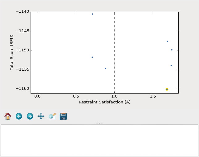
A screenshot of the plot_funnels GUI.

Remember that the purpose of this step is to generate physically realistic models with the geometry we want to design. These two goals are somewhat at odds with each other, in the sense that models that are less physically realistic should be able to achieve more ideal geometries. The second command displays a score vs. restraint satisfaction plot that we can use to judge how wells these two goals were balanced. If too many models superimpose with the restraints too well, the restraints might too strong. If too few models get within 1Å of the restraints, they might be to weak. You can tune the weights of the restraints by manually editing shared_defs.xml.

Stabilize good backbone models

The next step in the pipeline is to select a limited number of backbone models to carry forward and to generate a number of designed sequences for each of those models. It’s worth noting that the first step in the pipeline already did some design, so the purpose of this step is more to quickly generate a diversity of designs than to introduce mutations for the first time.

The following command specifies that we want to carry forward any model that puts its Glu within 1.0Å of where we restrained it to be:

$ pull_into_place 04 rescue_ksi_d38e 1 'restraint_dist < 1.0'
Selected 4 of 8 models

Note

This command just makes symlinks from the output directory of the model building command to the input directory of the design command. The models that aren’t selected aren’t deleted, and you run this command more than once if you change your mind about which models you want to keep.

This is a very relaxed threshold because we used --test-run in the previous step and don’t have very many models to pick from. For a production run, I would try to set the cutoff close to 0.6Å while still keeping a couple thousand models. You can also eliminate models based on total score and a number of other metrics; use the --help flag for more information.

Also note that we had to specify the round “1” after the name of the workspace. In fact, most of the commands from here on out will expect a round number. This is necessary because, later on, we will be able to start new rounds of design by picking models from the results of validation simulations. We’re currently in round 1 because we’re still making our first pass through the pipeline.

Once we’ve chosen which models to design, we need to push that information to the cluster:

$ pull_into_place push rescue_ksi_d38e

Then we can log into the cluster and start the design simulations:

$ ssh chef.compbio.ucsf.edu
$ pull_into_place 05 rescue_ksi_d38e 1 --test-run
$ exit

With the --test-run flag, this step should take about 30 min. When the design simulations are complete, we can download the results to our workstation as before:

$ pull_into_place fetch_data rescue_ksi_d38e

Validate good designs

You could have hundreds of thousands of designs after the design step, but it’s only really practical to validate about a hundred of those. Due to this vast difference in scale, picking which designs to validate is not a trivial task.

PIP approaches this problem by picking designs with a probability proportional to their Boltzmann-weighted scores. This is naive in the sense that it only considers score (although we are interested in considering more metrics), but more intelligent than simply picking the lowest scores, which tend to be very structurally homogeneous:

$ pull_into_place 06_pick rescue_ksi_d38e 1 -n5
Total number of designs:       39
    minus duplicate sequences: 13
    minus current inputs:      13

Press [enter] to view the designs that were picked and the distributions that
were used to pick them.  Pay particular attention to the CDF.  If it is too
flat, the temperature (T=2.0) is too high and designs are essentially being
picked randomly.  If it is too sharp, the temperature is too low and only the
highest scoring designs are being picked.

Accept these picks? [Y/n] y
Picked 5 designs.

This command will open a window to show you how the scores are distributed and which were picked. As the command suggests, it worth looking at the cumulative distribution function (CDF) of the Boltzmann-weighted scores to make sure it’s neither too flat nor too sharp. This is a subjective judgment, but one good rule of thumb is that the designs being picked (represented by the circles) should be mostly, but not exclusively, low-scoring. The CDF below looks about like what you’d want:

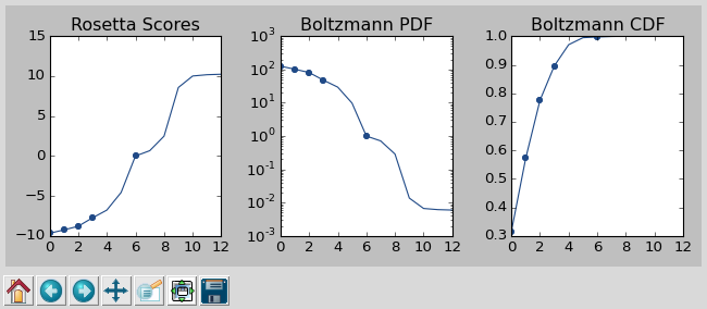
A screenshot of the 06_pick_designs_to_validate GUI.

The -n5 argument instructs PIP to pick 5 designs to validate. The default is 50, which would be appropriate for a production run. However, in this demo we only have about 50 designs because we’ve been using the --test-run flag. The algorithm that picks from a Boltzmann weighted distribution gets very slow when the number of designs to pick is close to the number of designs to pick from, which is why we only pick 5.

It’s also worth noting that there is a 06_manually_pick_designs_to_validate command that you can use if you have a PDB file with a specific mutation (perhaps that you made in pymol) that you want to validate. This is not normally part of the PIP pipeline, though:

$ pull_into_place 06_man rescue_ksi_d38e 1 path/to/manual/design.pdb

We can push our picks to the cluster in the same way as before:

$ pull_into_place push rescue_ksi_d38e

The validation step consists of 500 independent loop modeling simulations for each design, without restraints. As with the model building step, the default algorithm is KIC with fragments and we need to create fragment libraries before we can start the simulations:

$ ssh chef.compbio.ucsf.edu
$ pull_into_place 07 rescue_ksi_d38e 1

Once the fragment libraries have been created (as before, this should take about an hour), we can run the validation simulations:

$ pull_into_place 08 rescue_ksi_d38e 1 --test-run
$ exit

We could wait for the simulations to finish (which as before will take about 30 min) then download the results to our workstation using the same fetch_data command as before. However, I generally prefer to use the following command to automatically download and cache the results from the validation simulations as they’re running:

$ pull_into_place fetch_and_cache rescue_ksi_d38e/03_validated_designs_round_1/outputs --keep-going

The simulations in production runs generate so much data that it can take several hours just to download and parse it all. This command gets rid of that wait by checking to see if any new data has been generated, and if it has, downloading it, parsing it, and caching the information that the rest of the pipeline will need to use. The --keep-going flag tells the command to keep checking for new data over and over again until you hit Ctrl-C, otherwise it would check once and stop.

Once we’ve downloaded all the data, we can use the plot command again to visualize the validation results:

$ pull_into_place plot rescue_ksi_d38e/03_validated_designs_round_1/outputs/*

The plot GUI has a number of features that can help you delve into your simulation results and find good designs. First, notice that there is a panel on the left listing all of the designs that were validated. You can click on a design to view the results for that design. You can also hit j and k to quickly scroll through the designs.

Second, notice that there is a place to take notes on the current design below the plot. The search bar in the top left can be used to filter designs based on these notes. One convention that I find useful is to mark designs with +, ++, +++, etc. depending on how much I like them, so I can easily select interesting designs by searching for the corresponding number of + signs.

Third, you can view the model corresponding to any particular point by right-clicking (or Ctrl-clicking) on that point and choosing one of the options in the menu that appears. For example, try choosing “Compare to wildtype”. Behind the scenes, this runs the compare_to_wildtype.sho script that we copied into the workspace with the path to the selected model as the first and only argument. That script then runs pymol with the design superimposed on the wildtype structure, a number of useful selections pre-defined, the proteins rendered as cartoons, the ligands rendered as sticks, and the camera positioned with a good vantage point of the active-site loop.

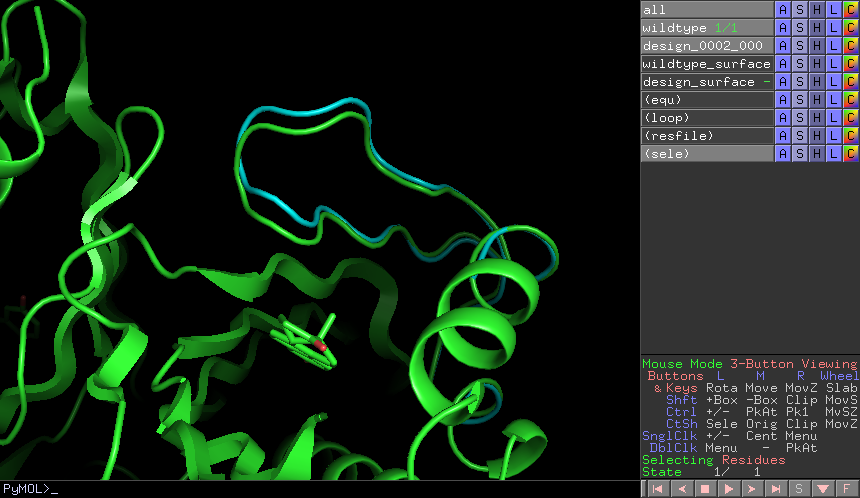
A screenshot of the pymol scene created by compare_to_wildtype.sho.

Within pymol, I use a plugin I wrote called wt_vs_mut to see how the design model differs from the wildtype structure. The plugin’s philosophy is to focus on each mutation one-at-a-time, to try to understand what interactions the wildtype residue was making and how those interactions are (or are not) being accommodated by the mutant residue. If this sounds useful to you, visit this page for instructions on how to install and use wt_vs_mut. “Compare to wildtype” pre-loads a shortcut to run wt_vs_mut with the correct arguments, so once you have the plugin installed, you can simply type ww to run it.

The plot command has several other features and hotkeys that aren’t described here, so you may find it worthwhile to read its complete help text:

$ pull_into_place plot --help

Iterate the design process

Often, some of the models from the validation simulations will fulfill the design goal really well despite not scoring very well. These models are promising because they’re clearly capable of supporting the desired geometry, and they may just need another round of design to make the conformation in question the most favorable.

You can use the 04_pick_models_to_design command to pick models from the validation simulations to redesign. The command has exactly the same form as when we used it after the model building step, we just need to specify that we’re in round 2 instead of round 1:

$ pull_into_place 04 rescue_ksi_d38e 2 'restraint_dist < 1'

I won’t repeat the remaining commands in the pipeline, but they’re exactly the same as before, with the round number updated as appropriate.

For a production run, I would recommend doing at least two rounds of design. I believe that models from the validation simulations – which are the basis for the later rounds of design – are more relaxed than the initial models, which makes them better starting points for design. At the same time, I would recommend against doing more than three or four rounds of design, because iterated cycles of backbone optimization and design seem to provoke artifacts in Rosetta’s score function.

Pick designs to test experimentally

The final step in the PIP pipeline is to interpret the results from the validation simulations and to choose an experimentally tractable number of designs to test. The primary results from the validation simulations are the score vs. restraint satisfaction plots. Promising designs will have distinct “funnels” in these plots: the models with the best geometries (i.e. restraint satisfaction) will also be the most stable (i.e. Rosetta score).

However, there are other factors we might want to consider as well. For example, you might be suspicious of designs with large numbers of glycine, proline, or aromatic mutations. You might also want to know which designs are the most similar to each other – either in terms of sequence or structure – so you can avoid wasting time testing two designs that are nearly identical. Finally, you might be interested in some of general-purpose metrics of protein stability that are not well represented by score alone, like the number of buried unsatisfied H-bonds or the amount of strain in the designed sidechains.

The following command generates a spreadsheet that collects all this information in one place:

$ pull_into_place 09 rescue_ksi_d38e 1

This command will create a file called quality_metrics.xlsx that you can open with Excel or any other spreadsheet program. By default, the spreadsheet will only include entries for designs where the lowest scoring model is within 1.2Å of satisfying the restraints. Each column presents a different quality metric, and each cell is colored according to how favorable that value of that metric is. The precise meaning and interpretation of each metric is discussed below:

Resfile Sequence

Show the amino acid identity of every position that was allowed to mutate in the design (although not all of the positions are necessarily different from wildtype). Use this information to look for specific sequence motifs that make you suspicious.

Sequence Cluster

Show which designs have the most similar sequences. Only positions that were allowed to design are considered in this clustering, and no alignment is done. The sequences are simply compared using a score matrix like BLOSUM80. Use this metric to avoid picking too many designs that are too similar to each other.

Struct Cluster

Show which designs are the most structurally similar. This metric works by creating a hierarchical clustering of the lowest scoring models for each design based on loop backbone RMSD. Clusters are then made such that every member in every cluster is within a certain loop RMSD of all its peers. Use this metric to avoid picking too many designs that are too similar to each other.

Restraint Dist (Å)

Show how well each design satisfies the design goal, as embodied by the restraints given at the very beginning of the pipeline.

Score Gap (REU)

Show the difference in score between the lowest scoring models with restraint distances less than and greater than 1Å and 2Å, respectively. Use this metric to get a rough idea of how deep the score vs. RMSD funnel is for each design.

% Subangstrom

Show what percent of the models from the validation simulations had sub-angstrom restraint distances. Use this metric to get a rough idea of how well-populated the score vs. RMSD funnel is.

# Buried Unsats

Show how many buried unsatisfied H-bonds each design has, relative to the input structure given at the very beginning of the pipeline. This is something that’s not accounted for by the Rosetta score function, but that can do a very good job discriminating reasonable backbones from horrible ones.

Dunbrack (REU)

Show the Dunbrack score for each residue that was part of the design goal (i.e. was restrained in the building step). High Dunbrack scores indicate unlikely sidechain conformations.